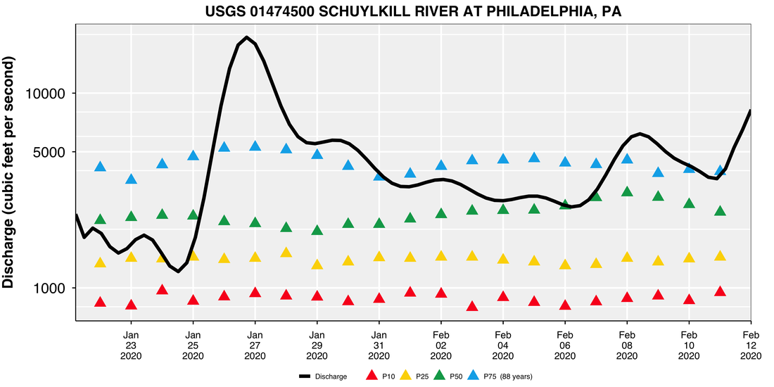
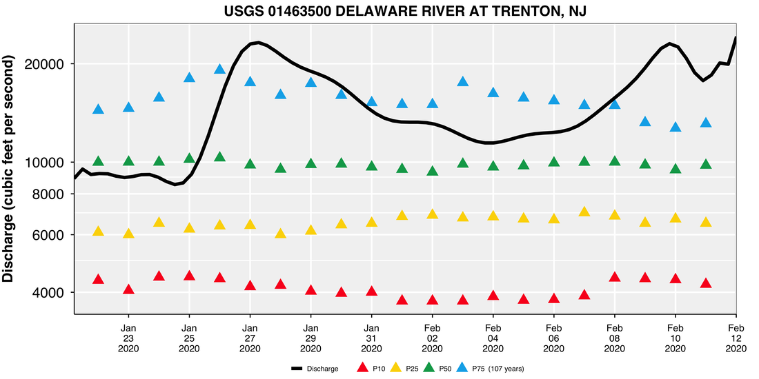
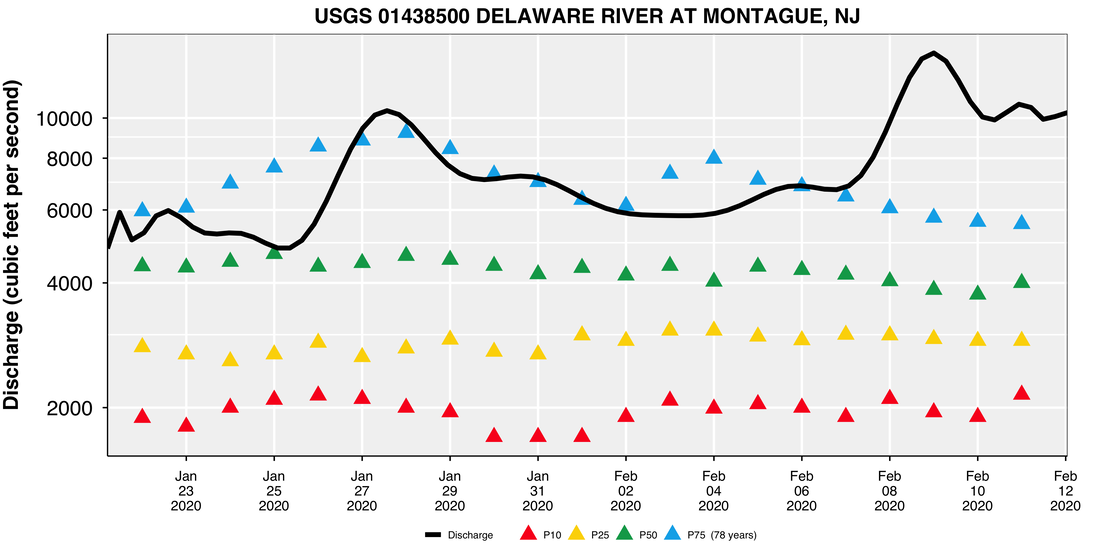
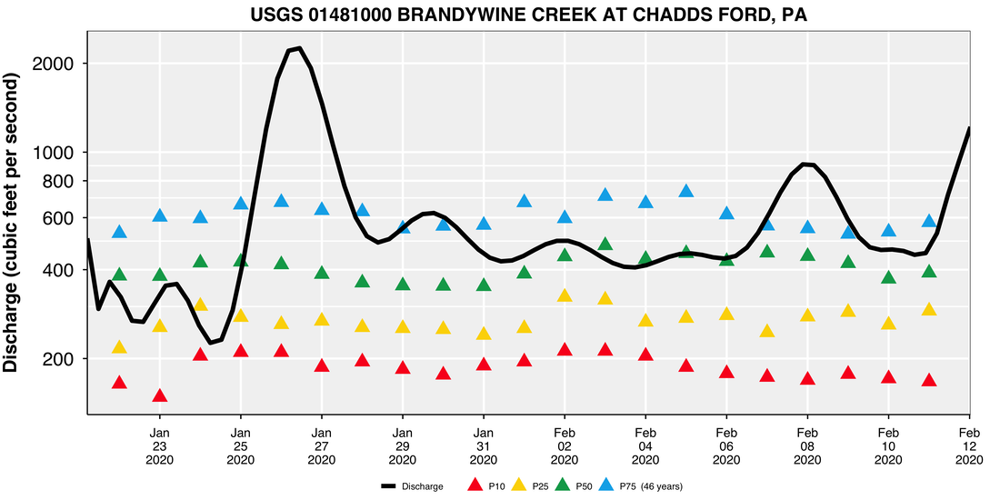
    library(dataRetrieval) library(scales) library(lubridate) library(tidyverse) # log scale tick marks and/or grid #' @param n Approximate number of ticks to produce #' @param NumBase Logarithm base logTicks <- function(n = 5, base = 10){ ##n indicated number of logarithm base ticks marks. e.g., base 10: 1, 2, 5, 10. divisors <- which((base / seq_len(base)) %% 1 == 0) mkTcks <- function(min, max, NumBase, divisor){ f <- seq(divisor, base, by = divisor) return(unique(c(base^min, as.vector(outer(f, base^(min:max), `*`))))) } function(x) { rng <- range(x, na.rm = TRUE) lrng <- log(rng, base = base) min <- floor(lrng[1]) max <- ceiling(lrng[2]) tck <- function(divisor){ t <- mkTcks(min, max, NumBase, divisor) t[t >= rng[1] & t <= rng[2]] } # produce a set of ticks and count how many ticks tcks <- lapply(divisors, function(d) tck(d)) l <- vapply(tcks, length, numeric(1)) # Take the set of ticks which is nearest to the desired number of ticks i <- which.min(abs(n - l)) if(l[i] < 2){ ticks <- pretty(x, n = n, min.n = 2) }else{ ticks <- tcks[[i]] } return(ticks) } } themebox <- function(base_family = "sans", ...){ theme_bw(base_family = base_family, ...) + theme( plot.title = element_text(size = 18, face = "bold", hjust=0.5), #plot.background = element_rect(fill = '#D6D5C9') #area not in the plot #panel.border = element_line(), panel.background = element_rect(fill="gray95", colour = "black"), panel.grid.major = element_line(size=0.95, linetype = 'solid',colour = "white"), panel.grid.minor = element_line(size=0.6, linetype = 'solid',colour = "white"), axis.ticks.length = unit(.15, "cm"), #spacing of axis text to plot panel; negative value closer to panel axis.ticks = element_line(colour = 'black',size=.60), axis.title = element_text(face="bold", size=18), axis.text.x=element_text(margin=unit(c(0.3,0.3,0.3,0.3), "cm"),colour="black", size = 12), axis.text.y=element_text(margin=unit(c(0.3,0.3,0.3,0.3), "cm"),colour="black", size = 18), axis.line = element_line(size=0.5, colour = "black"), #axis.ticks.x = element_blank(), legend.position="bottom", legend.box = "horizontal", #legend.background = element_blank(), #legend.margin=margin(0,0,0,0), #legend.title=element_blank() legend.box.margin=margin(-15,-10,-1,-10), legend.title=element_text(size=9), plot.margin = margin(0.25, 1, 0.01, 0.1, "cm") #(top,right,bottom,left), #aspect.ratio = .2, ) } Today<-as.POSIXlt(Sys.Date()) Today<-as.POSIXlt(Today) unlist(unclass(Today)) Today$mday <- Today$mday Today<-as.Date(Today) Year<-format(Sys.Date(), "%Y") site_no<-c('01463500', '01438500','01474500','01481000') site_name<-c('TRENTON, NJ', 'MONTAGUE, NJ', 'PHILADELPHIA, PA', 'CHADDS FORD, PA') river_name<-c('DELAWARE RIVER', 'DELAWARE RIVER', 'SCHUYLKILL RIVER', 'BRANDYWINE CREEK') file_name<-c('Trenton','Montague','Schuylkill','ChaddsFord') Dashboard<-data.frame(site_no, site_name, river_name, file_name) for (i in 1:nrow(Dashboard)){ png(file=paste0(Dashboard$file_name[i],".png"), width = 4000, height = 2000, res=300) Stats <- readNWISstat(siteNumbers = Dashboard$site_no[i],parameterCd = "00060", statReportType="daily", statType=c("p10","p25","p50","p75")) Stats <- readNWISstat(siteNumbers = Dashboard$site_no[i],parameterCd = "00060", statReportType="daily", statType=c("p10","p25","p50","p75")) Stats$MonthDay <- with(Stats, paste(month_nu, day_nu, sep="-")) FirstDate= Today-21 LastDate= Today DateFill<-c(FirstDate, LastDate) NewTimeSeries<-as.data.frame(DateFill) NewTimeSeries<- NewTimeSeries %>% mutate(DateFill = as.Date(DateFill)) %>% complete(DateFill = seq.Date(min(DateFill), max(DateFill), by="day")) NewTimeSeries$Year<-year(NewTimeSeries$DateFill) NewTimeSeries$Month<-month(NewTimeSeries$DateFill) NewTimeSeries$Day<-mday(NewTimeSeries$DateFill) NewTimeSeries $MonthDay <- with(NewTimeSeries, paste(Month, Day, sep="-")) Update<-right_join(Stats, NewTimeSeries, by = c("MonthDay", "MonthDay")) Update$Ymd <- as.Date(with(Update, paste(Year, Month, Day, sep="-")), "%Y-%m-%d") Update$dateTime<-as.POSIXct(Update$Ymd,tz="UTC") NOW<-readNWISuv(siteNumbers= Dashboard$site_no[i], parameterCd=c("00060"), startDate = Today-21, endDate = Today) OUTPUT<-right_join(Update, NOW, by = c("dateTime", "dateTime")) OUTPUT<-OUTPUT%>% select(21,23,24,10:14) colnames(OUTPUT)<-c("dateTime","site_no","X_00060_00000","count_nu","p10_va","p25_va","p50_va","p75_va") data_long <- gather(OUTPUT, PercentileName, PercentileValue, p10_va:p75_va, factor_key=TRUE) as.numeric(data_long$count_nu) All<-ggplot(data_long, mapping=aes(x=dateTime, y=X_00060_00000)) + geom_point(mapping=aes(x=dateTime, y=PercentileValue, color=factor(PercentileName)),size = 5, shape=17)+ stat_smooth(mapping=aes(x = dateTime, y = X_00060_00000, fill='Discharge'), method = "lm", formula = y ~ poly(x, 21), se = FALSE, size=2, color="black") + scale_y_log10(name = 'Discharge (cubic feet per second)', breaks = logTicks(n = 4), #1,2,4,10,100, etc. outline how many major base pair ticks marks minor_breaks = logTicks(n=10))+ scale_x_datetime(breaks = date_breaks("2 day"),labels = date_format("%b\n%d\n%Y"), name=NULL, minor_breaks = NULL, expand = c(0, 0))+ ggtitle(paste0("USGS ",Dashboard$site_no[i], " ",Dashboard$river_name[i], " AT ", Dashboard$site_name[i]))+ themebox()+ labs(color=paste0("(",mean(data_long$count_nu,na.rm=TRUE)," years)"))+ scale_fill_manual("",values=c("#171A21"))+ scale_linetype_manual(values=c("solid"))+ scale_shape_manual(values = c(17, 17, 17, 17))+ scale_color_manual(labels=c("P10","P25","P50","P75"), values=c("#FA2121","#FCD600","#01A558","#00AFEA"))+ ##FBB02D orange guides(fill = guide_legend(order = 1), colour = guide_legend(title.position = "right")) print(All) dev.off() } graphics.off() All
1 Comment
|
Archives
February 2020
Categories |
||
 RSS Feed

@ 2016 Evan Kwityn. All Rights Reserved