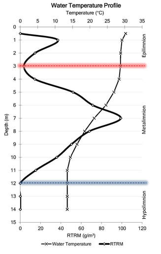
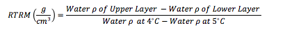
Relative Thermal Resistance to Mixing (RTRM)

When observing physical water characteristics in the ocean, lakes, ponds, or rivers energy (i.e., heat) is often gained or lost from the surface and is transported with depth. Since water temperatures change the density of water, cold water has greater density compared to warm water. Observing water temperatures through depth gives us important information that deals with a range of water temperatures.

There are three categories that illustrate the formation of a water column that are divided in this concept due to density. These categories include the epilimnion (upper layer), thermocline or metalimnion (middle layer), and the hypolimnion (bottom layer). Determining these layers throughout a water column is often important when identifying where organisms reside and are most productive. This is important since water temperature and metabolic rate are correlated.

---

Relative thermal resistance to mixing is able to quantify stratification as a function of temperature differential, exact position of the thermocline, the exact width of the metalimnion, and how stable of stratification results from an non linear change. RTRM identifies a relatively easy computation. Instead of visually trying to identify stratification this method can be utilized to identify both the location and intensity of thermal stratification.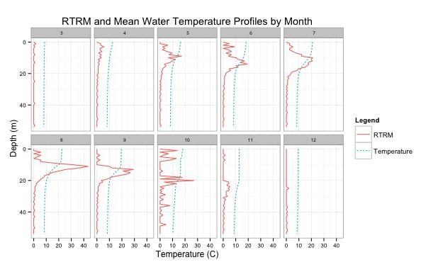 

#https://github.com/EvanAquatic
#Function to calculate water density (mg/m^3) from water temperature (celsius)
WaterDensityCalc <- function(x) { 
  Density=(1000*(1-((Temperature+288.9414)/(508929.2*(Temperature+68.12963)))*(Temperature-3.9863)^2)/1000) #output is water density in mg/m^3
}

Depth=Profile$Sample.Depth 
Temperature=Profile$Temperature
Water_Density<-WaterDensityCalc(Temperature) ###Calculating water density from the defined function  

RTRM<-data.frame(Profile$Sampling.Location, Depth, Temperature, Water_Density) ###Creating dataframe with outputs

##Calculate RTRM
RTRM$RTRM_OUTPUT= NA
for(i in seq(1, nrow(RTRM))){
  RTRM[i,"RTRM_OUTPUT"] = RTRM[i,"RTRM_OUTPUT"] = ((RTRM[i+1,"Water_Density"] - RTRM[i,"Water_Density"])/(1-0.9999919))
}

#1000*(1-((4+288.9414)/(508929.2*(4+68.12963)))*(4-3.9863)^2)/1000=1
#1000*(1-((5+288.9414)/(508929.2*(5+68.12963)))*(5-3.9863)^2)/1000=0.9999919

RTRM$RTRM_OUTPUT[RTRM$RTRM_OUTPUT<0]<-0 #Removing negative values
RTRM

#######General Plots and Figures
library(ggplot2)
library(MASS)
library(reshape)
library(reshape2)

#Incorporating influences of month or date
#RTRM$NewDate <- format(as.Date(RTRM$RTRM1.Date, format="%m/%d/%Y"), "%Y/%m")
#RTRM$Monthday <- format(as.Date(RTRM$RTRM1.Date, format="%m/%d/%Y"), "%m/%d")

###################
#Creating new dataframes to plot water temperature and RTRM
df<-data.frame(RTRM$Profile.Sampling.Location, RTRM$Depth, RTRM$Temperature, RTRM$RTRM_OUTPUT)
names(df)<-c("SampleLocation", "Depth", "Temperature", "RTRM") #New datadrame output with new header names; length=lt and weight=wt
newdf<- melt(df, id = c("SampleLocation","Depth"))
names(newdf)<-c("SampleLocation", "Depth", "Legend", "Output") #New datadrame output with new header names; length=lt and weight=wt

###Water Temperature and RTRM Profile Plot Outputs
g<-ggplot(newdf, aes(x=Output, y =Depth, color=Legend))+
  theme_bw() + 
  geom_path(aes(linetype=Legend),linejoin = 'round', size=1 ) + 
  facet_wrap(~SampleLocation, ncol=5)+
  # facet_grid(Collection.Date.ymd~Collection.Year)+
  labs(title='4/26/2018  Reservoir Relative Thermal Resistance to Mixing (RTRM) and Water Temperature Profiles')+
  xlab("Temperature (C) and RTRM (g/m^3)")+
  ylab("Depth (m)")+
  scale_x_continuous(limits=c(0,30), expand=c(0,0))+
  scale_y_reverse(breaks=seq(12,0, by=-1), limits=c(12,0), expand=c(0,0)) +
  theme(strip.text = element_text(size=6.5, lineheight=0.1, hjust=0.5),
        axis.text.y = element_text(size=8, colour="black"),
        axis.text.x = element_text(size=8, colour="black"), 
        panel.spacing = unit(1, 'lines'), 
        legend.position = "top", legend.background = element_rect(color = "black", 
         size = .1), legend.direction = "horizontal")

###################
#Creating new dataframes to plot Dissolved Oxygen, pH, % Dissolved Oxygen, etc. 
df2<-data.frame(Profile$Sampling.Location, Profile$Sample.Depth, Profile$Dissolved.Oxygen)
names(df2)<-c("SampleLocation", "Depth", "Dissolved Oxygen") #New datadrame output with new header names; length=lt and weight=wt
newdf2<- melt(df2, id = c("SampleLocation","Depth"))
names(newdf2)<-c("SampleLocation", "Depth", "Legend", "Output") #New datadrame output with new header names; length=lt and weight=wt
​
###Dissolved Oxygen Profile Plot Outputs
g<-ggplot(newdf2, aes(x=Output, y =Depth, color=Legend))+
  theme_bw() + 
  geom_path(aes(linetype=Legend), size=1 ) + 
  facet_wrap(~SampleLocation, ncol=5)+
  # facet_grid(Collection.Date.ymd~Collection.Year)+
  labs(title='4/26/2018 Reservoir Dissolved Oxygen Profiles')+
  xlab("Dissolved Oxygen (mg/L)")+
  ylab("Depth (m)")+
  scale_x_continuous(limits=c(0,12), expand=c(0,0))+
  scale_y_reverse(breaks=seq(12,0, by=-1), limits=c(12,0), expand=c(0,0)) +
  theme(strip.text = element_text(size=6.5, lineheight=0.1, hjust=0.5),
        axis.text.y = element_text(size=8, colour="black"),
        axis.text.x = element_text(size=8, colour="black"), 
        panel.spacing = unit(1, 'lines'), 
        legend.position = "top", legend.background = element_rect(color = "black", 
        size = .5), legend.direction = "horizontal")

​[1] Kortmann, R.W. 1990. Thermal Stratification in Reservoirs: Causes, Consequences, Management Techniques.  Proceedings  AWWA-WQTC, San Diego, November 1990.